Backpropagation and Gradient Descent: How Neural Networks Learn From Errors
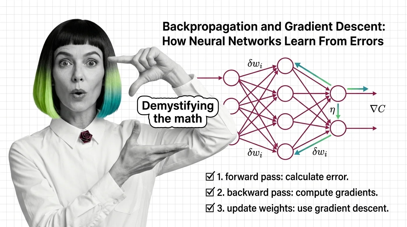
Table of Contents
ELI5
A neural network guesses, measures how wrong it was, then backpropagation sends that error backward through every layer so each weight learns exactly how much to change.
A Neural Network Basics for LLMs with a hundred million parameters produces the wrong output. Somewhere in that stack of matrices, some weights contributed more to the mistake than others. The network identifies them — and corrects them by the right amount — in a single backward pass through the computation graph, using one principle from introductory calculus. That principle is the chain rule, and the algorithm built on it has been training every neural network you have heard of since 1986.
The Error Signal That Flows Backward
Training means adjusting weights until outputs match targets. The adjustment itself is trivial — add or subtract a small number. The hard part is attribution: a deep network might have dozens of layers between input and output, each transforming the signal through nonlinear functions. When the final answer is wrong, which weights in which layers are responsible, and by how much?
Backpropagation solves this by running the computation in reverse.
How does backpropagation work step by step in neural network training
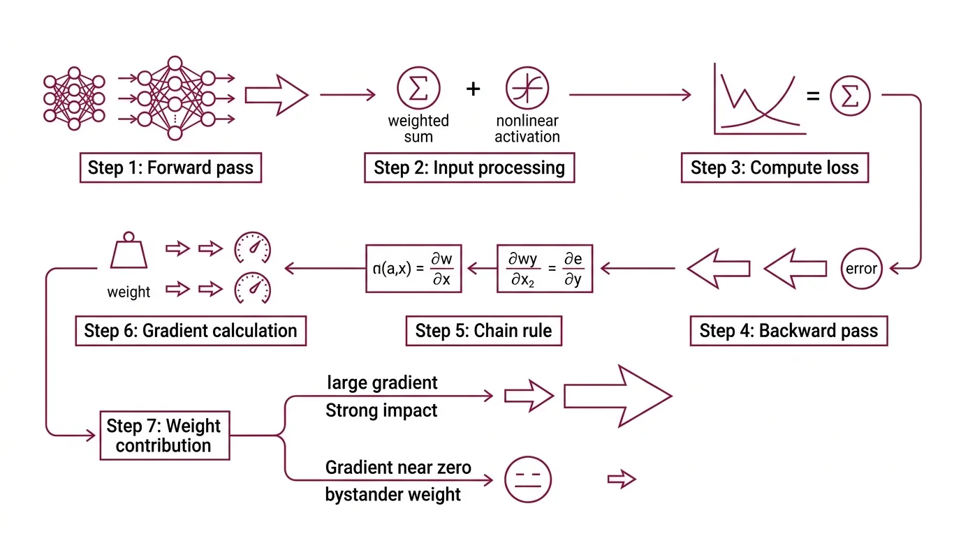
The forward pass pushes data through the network layer by layer. Each neuron computes a weighted sum of its inputs, applies a nonlinear activation function, and passes the result to the next layer. At the output, a loss function — cross-entropy for classification, mean squared error for regression — quantifies the distance between prediction and reality.
The backward pass starts where the forward pass ended. From the loss, the algorithm computes how sensitive that loss is to each weight in the final layer. Then it applies the chain rule to propagate those sensitivities backward through every preceding layer. Each weight receives a gradient — a number that says precisely how much the total loss would change if that weight were nudged by a small amount.
Weights with large gradients contributed significantly to the error. Weights with gradients near zero were bystanders.
Rumelhart, Hinton, and Williams formalized this mechanism — the chain rule, applied backward — in their 1986 paper (Nature). The same algorithm, the same math, now running through models with hundreds of billions of parameters. What changed is the scale. The principle has not been revised.
The Calculus That Carries the Algorithm
The word “calculus” deters people who should not be deterred. Gradient Descent requires gradients, and gradients require derivatives — but the toolkit is smaller than it appears.
What math do you need to understand backpropagation and gradient descent
Three concepts carry the load.
Partial derivatives. A network’s loss depends on all its weights simultaneously. A partial derivative isolates the effect of one weight while treating the rest as constants. If you can differentiate a single-variable function, extending to partial derivatives is largely a change in notation — the core idea is identical.
The chain rule. A neural network is a composition of functions — layers nested inside layers. The chain rule decomposes the derivative of the final output with respect to any interior weight into a product of local derivatives. Each layer computes its own local gradient; everything upstream arrives from the layer above. Backpropagation is the chain rule applied systematically — nothing more exotic, nothing less powerful.
Linear algebra. Weights are matrices. Inputs are vectors. A forward pass through a single layer is a matrix multiplication followed by a nonlinearity. Understanding matrix dimensions, dot products, and how a vector transforms under a linear map is sufficient to follow the standard backpropagation equations without difficulty.
Anything beyond this — Jacobians, Hessians, second-order methods — belongs to advanced optimization theory, not to understanding how backpropagation works.
Modern frameworks have automated the derivative computation entirely.
PyTorch’s autograd engine builds a dynamic directed acyclic graph during the forward pass and computes gradients via vector-Jacobian products, rebuilding the graph after each .backward() call (PyTorch Tutorials). You define the forward computation; the framework derives the backward pass. This is automatic differentiation — the reason researchers spend their time on architecture design rather than gradient derivation.
Three Ways to Walk Down a Loss Surface
Backpropagation gives you the gradient — the direction of steepest descent on the loss surface. The remaining question is practical: how many training examples should inform each step, and how frequently should you recalculate?
What is the difference between batch stochastic and mini-batch gradient descent
Batch gradient descent computes the gradient over the entire training dataset before updating a single weight. The direction is precise — averaged over every example, the gradient points reliably toward lower loss. The cost, however, is proportional to dataset size, which for modern training sets means a single update can take unreasonably long.
Stochastic gradient descent takes the opposite approach: compute the gradient from one training example and update immediately. Each step is fast but noisy — a single example might push the weights in a direction that helps for that sample but hurts overall. Over thousands of steps the noise averages out, but the path to convergence is jagged and unpredictable.
Mini-batch gradient descent occupies the middle ground. Sample a batch — sizes typically range from tens to several thousand, depending on hardware and model — compute the gradient over that batch, and update. Mini-batches reduce gradient variance compared to pure stochastic descent; the reduction grows with the square root of the batch size (D2L). Convergence is smoother, and each update costs far less than a full-dataset pass.
Not a compromise. A deliberate engineering choice.
In practice, mini-batch is the quiet default for LLMs. The Adam Optimizer, introduced by Kingma and Ba (Kingma & Ba), pairs mini-batch gradients with per-parameter adaptive learning rates and momentum estimates. Its variant AdamW — which decouples weight decay from the adaptive rate — is the default optimizer for virtually every transformer architecture in production: GPT, Llama, Gemma, Mistral, and vision transformers (Lightly AI).
What the Gradient Reveals — and Where It Disappears
A gradient encodes more than a direction. Its magnitude at each weight tells you how sensitive the loss is at that point in the network — steep surface means a small weight change produces a large effect; flat surface means the weight is near an optimum or trapped in a region where learning has stalled.
Increase the learning rate and the network steps farther along the gradient per update: faster convergence, but overshooting the minimum becomes likely. Decrease it and the network inches forward so slowly that training stalls before reaching a useful solution. If you see training loss oscillating wildly, the learning rate is probably too high. If the loss curve flatlines early, it may be too low.
Stack many layers with sigmoid or tanh activations and a different failure emerges. Gradients shrink exponentially as they propagate backward — by the time the error signal reaches the earliest layers, it is indistinguishable from zero. Those layers stop learning entirely. This is the Vanishing Gradient problem, and it constrained useful network depth for decades.
The solutions are architectural: ReLU activations that avoid saturation, Xavier or Kaiming initialization that keeps gradient magnitudes stable across depth, batch normalization that rescales layer activations, and residual connections that give the gradient a shortcut path through the network.
Rule of thumb: if your network trains the last few layers effectively but the first layers barely change, suspect vanishing gradients before investigating anything else.
When it breaks: Backpropagation requires every operation in the computation graph to be differentiable. When the graph includes discrete decisions — hard attention masks, sampling from a categorical distribution, non-differentiable thresholds — the gradient is undefined at those points, and the error signal cannot pass through. Workarounds exist (straight-through estimators, Gumbel-softmax relaxation), but they are approximations with their own failure modes.
Security & compatibility notes:
- PyTorch TorchScript: Deprecated as of PyTorch 2.6. For model export and tracing, migrate to
torch.export.- PyTorch
torch.load: The defaultweights_onlyparameter changed for security reasons. Existing code usingtorch.loadwithout explicitweights_only=Truemay behave differently after upgrading.
The Data Says
Backpropagation is not a learning theory — it is a bookkeeping algorithm for partial derivatives, applied recursively through a computation graph. Gradient descent is the step that algorithm enables: adjusting each weight in the direction that reduces the loss. Every large language model you interact with was trained by this pair. The math is four decades old. The principle has not been replaced. The only thing that scales alongside the models is the compute required to run the chain rule through billions of parameters.
AI-assisted content, human-reviewed. Images AI-generated. Editorial Standards · Our Editors