Adjacency Matrices, Node Features, and the Prerequisites for Understanding Graph Neural Networks

Convolutional networks see pixel grids. Transformers see token sequences. Both assume the data has a fixed spatial or temporal order — and both break the moment your data is a molecule, a social network, or a Knowledge Graph where the structure itself carries the meaning. Graph Neural Networks were built for exactly this case: data where relationships are irregular, the number of neighbors varies per node, and no canonical ordering exists. The question worth asking is not what GNNs can do — that list grows weekly. The question is: what mathematical objects does a GNN actually consume, and what do you need to understand before the architecture makes sense?

How a Matrix of Zeros and Ones Becomes a Neural Network’s Map

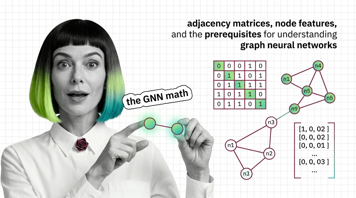
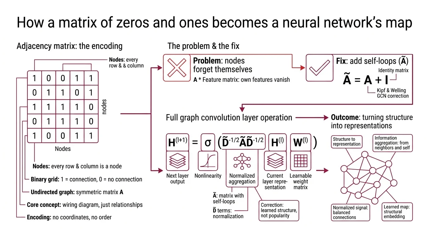
Think of an adjacency matrix as the wiring diagram for a circuit — except instead of recording which components connect through which traces, it records which nodes share an edge in a graph. Every row is a node. Every column is a node. A 1 at position (i, j) means node i and node j are connected; a 0 means they are not.

That is the entire encoding. No coordinates, no pixel positions, no word order. Just a binary grid of relationships.

What is an adjacency matrix and how do GNNs use it?

The adjacency matrix A is an n x n binary matrix where n is the number of nodes in the graph. For undirected graphs, A is symmetric: if node 3 connects to node 7, then node 7 connects to node 3.

But raw adjacency matrices create a problem for neural networks. When you multiply A by a feature matrix, a node’s own features vanish from the computation — it aggregates information from its neighbors but forgets itself. The fix is self-loops: the modified matrix A-tilde = A + I adds the identity matrix so that every node counts as its own neighbor — a correction introduced in the original GCN formulation (Kipf & Welling).

The full Graph Convolution layer then becomes:

H^(l+1) = sigma(D-tilde^{-1/2} A-tilde D-tilde^{-1/2} H^(l) W^(l))

where D-tilde is the degree matrix of A-tilde, H^(l) is the node representation at layer l, W^(l) is a learnable weight matrix, and sigma is a nonlinearity (Kipf & Welling). The D-tilde terms normalize the aggregation — without them, high-degree nodes would dominate the signal simply by having more connections, drowning out the features of sparsely connected nodes.

This normalization is not a convenience. It is the difference between a network that learns structure and one that learns popularity.

But the adjacency matrix only tells you who is connected. What the network does with that connection — how it turns structure into learned representations — requires a different mechanism.

The Three-Step Conversation Between Nodes

If the adjacency matrix is the wiring diagram, Message Passing is the protocol nodes use to communicate. The MPNN framework reduces every GNN variant to three operations that repeat at each layer (Gilmer et al.).

What are the key components of a graph neural network architecture?

Three components define the architecture: the node feature matrix, the message-passing mechanism, and the aggregation function.

The node feature matrix X, an element of R^{n x d}, stores the initial representation of every node — n nodes, each described by d features. For a molecular graph, those features might encode atom type, charge, and hybridization state. For a citation network, they might be word embeddings of paper abstracts. X serves as the input layer H^(0) from which all subsequent representations are computed (Distill GNN Intro).

Message passing itself unfolds in three steps: gather the embeddings of each node’s neighbors; aggregate them using a permutation-invariant function — sum, mean, or max; then update the node’s own embedding through a learned transformation (Distill GNN Intro). The permutation invariance is the architectural commitment that matters most here — since graphs have no canonical node ordering, the aggregation must be order-independent. Reorder the neighbor list, and the output must remain identical.

The aggregation function is where architectural variants diverge. A standard GCN uses a normalized mean. A Graph Attention Network learns attention weights so that some neighbors contribute more than others — the network decides which connections carry the most relevant signal. Graphsage takes a different route: instead of aggregating all neighbors, it samples a fixed-size subset, making the computation tractable for graphs with millions of nodes.

Each variant solves a different engineering constraint, but all three share the same skeleton: gather, aggregate, update. What determines whether this skeleton produces insight or noise is the mathematical vocabulary it draws from.

The Linear Algebra That Makes Graphs Computable

GNN papers read like linear algebra textbooks because, at the computational level, they are. The architecture is inseparable from the math — and understanding where the math comes from makes the design choices legible rather than arbitrary.

What math do you need to understand graph neural networks?

Three branches of mathematics recur across GNN literature, roughly in order of necessity.

Matrix multiplication and linear algebra form the foundation. Every GNN layer is a matrix multiplication: the adjacency matrix (or its normalized variant) multiplied by the feature matrix, then multiplied by a learnable weight matrix. If you cannot read H^(l+1) = sigma(A-tilde H W) as “aggregate neighbor features, apply a linear transformation, pass through a nonlinearity,” the rest of the architecture will remain opaque.

Graph theory fundamentals — degree, adjacency, connected components, shortest paths — provide the vocabulary. The degree matrix D is diagonal, with D_ii counting node i’s connections. The graph Laplacian L = D - A captures the difference between a node’s own signal and the average of its neighbors; it functions as a discrete second derivative, measuring how much a signal at one node deviates from its local neighborhood.

Spectral Graph Theory connects GNNs to signal processing on graphs. The eigenvalues of the graph Laplacian define a frequency spectrum for signals on the graph — low eigenvalues correspond to smooth, slowly varying patterns; high eigenvalues correspond to rapid oscillations between adjacent nodes. Kipf and Welling’s GCN is, mathematically, a first-order approximation of spectral graph convolutions using Chebyshev polynomials (Kipf & Welling). The spectral derivation explains why the architecture works but is not required to use it — most practitioners treat GCN layers as a parameterized aggregation and never look at the eigenvectors.

The gap between “can use” and “understands why” lives in the spectral domain.

Depth, Frameworks, and the Ceiling You Will Hit

A GNN that stacks many layers should, in principle, capture information from increasingly distant nodes — each layer extends the receptive field by one hop. In practice, something more troubling happens.

After roughly two to six layers, node representations begin to converge. Distinct nodes start producing near-identical embeddings. The network loses its ability to distinguish between structurally different neighborhoods, and classification accuracy degrades. This is Oversmoothing — a phenomenon where repeated aggregation washes out local features until every node looks like the graph’s global average (Li et al.). The depth limit of two to six layers is a general guideline, not a hard boundary; recent work on graph rewiring and residual connections pushes usable depth further, but the fundamental tension between depth and distinguishability remains unresolved.

If you increase GNN depth, expect diminishing — and eventually negative — returns on node classification tasks. If you need long-range dependencies, consider architectures that aggregate without smoothing, such as attention-based models or graph transformers. If your graph has strong local structure but weak global patterns, shallow networks will outperform deep ones.

Rule of thumb: Start with two layers. Add a third only if validation performance improves. Beyond that, you are likely fighting oversmoothing rather than learning features.

When it breaks: GNNs struggle with graphs where the meaningful signal lives in long-range relationships — interactions between nodes five or more hops apart. The message-passing paradigm requires that many layers to propagate the signal, but oversmoothing degrades it before it arrives. This is not a tuning problem; it is a structural limitation of the aggregation mechanism.

On the tooling side, two frameworks dominate. Pytorch Geometric (PyG) v2.7.0, released October 2024, remains the most actively developed — supporting PyTorch 2.6 through 2.8 and adding a new torch_geometric.llm sub-package that bridges GNNs and language models (PyG GitHub). Deep Graph Library (DGL) v2.4.0, released September 2024, offers comparable functionality but its release cadence has slowed; at least one downstream project has cited inactivity and migrated to PyG (DGL GitHub).

Compatibility notes:

• PyG SparseTensor deprecation: SparseTensor from torch-sparse is being deprecated in favor of EdgeIndex/Index. Existing code using SparseTensor will need migration.
• DGL maintenance pace: DGL’s last release was September 2024. Evaluate release activity before committing to new projects.

The Data Says

Not a model architecture. A mathematical commitment to the idea that structure is data. The adjacency matrix, node features, and message-passing protocol form a closed system: if you understand how information propagates through a normalized matrix multiplication, you understand every GNN variant as a specific answer to the aggregation question. The prerequisite is not deep learning experience. It is comfort with linear algebra and the willingness to read a graph Laplacian as a frequency filter.